Drift
We define drift across two distributions of data if the behavior of the model is dissimilar (different) across both of those distributions. What's important is not just how your model's output differs when the distribution of data changes but also how its performance differs; most importantly, is it still accurate? This can happen when switching from one data split to another, but especially when transitioning from train-and-test data to out-of-time (OOT) or live production data. Such potential drift is typically due to one or more of three things:
- The original training data distribution was ill-suited to real-world use cases.
- The OOT distribution has time-shifted or is otherwise affected by considerations absent in the training data — factors like seasonality, expanded locations, drastic economic/environmental changes, etc.
- Some feature/variable properties (feature influences) are measurably different in the two distributions.
TruEra's drift analysis helps you identify consequential data drift in your models by (a) comparing the difference in model output behavior and accuracy across different time periods and data splits, and (b) pinpointing which features are driving the difference in behavior and accuracy.
Once the factor(s) promoting drift are identified, TruEra enables you to drill down and measurably assess specific differences in the data distributions of the feature and the affect this is having on the model's outcome.
How is data drift analyzed?
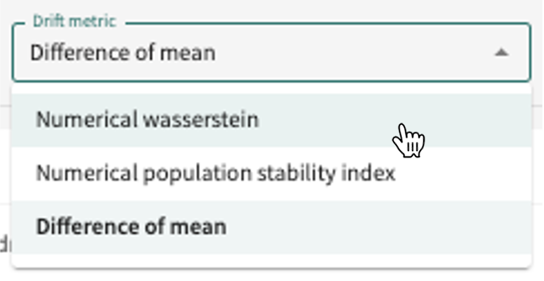
TruEra compares two data splits using the selected distributional difference metric — Wasserstein, PSI, or Difference of Mean — and plots overall model scores for each split, as well as performing a feature-by-feature comparison to determine the given feature's contribution to score, error, and feature value drift.
Wasserstein, also known as the Earth Mover's distance or EMD, is the "minimum amount of work" to match split-A with split-B, divided by the total weight of the split-A distribution. Population Stability Index (PSI) compares the distribution of the scoring variable in the OOT split to its distribution in the train/test split. Difference of Mean measures the absolute difference between the mean value in the two splits.
In order to understand drift, you'll want to provide a human-labeled random sampling of OOT data to compare with your train/test data, although any two splits defined for the project model can be compared.
How is drift calculated?
A Model Score Drift (MSD) metric captures the distributional difference of model scores between two splits. A high MSD signals that the models outputs have shifted. Depending on the situation, it may or may not be a cause for concern. It is worthwhile to understand the root causes of the shift to determine whether a model needs to be adjusted or not.
Meanwhile, a Feature Influence Drift (FID) metric captures the difference in influences between the train/test and OOT distributions for each feature. FID computes the difference between the two distributions of feature influences. A high FID indicates a strong feature influence contribution to model drift.
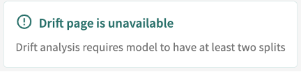
Important
TruEra's Drift functionality requires that you first upload at least two splits mapped to the currently selected model. If only one split or none exists for the current project model, you will receive the following warning:
Launching the Analysis
In addition to the selectable parameters — Base split, Compare split, and Drift Metric — your comparison options include:
- Filter by segment – narrows your focus by segment or a specific feature's relative value.
- Estimated accuracies – plots the estimated accuracy for a split in the absence of ground truth labels.
Note
Estimated accuracies assume that while the input X into a model may drift (data drift), the relationship between the input X and target variables Y does not change. A change in the relationship between input and target changes (concept drift) would indicate the need to retrain the underlying model to reflect the new relationship between X and Y. The estimated accuracy for a given slice of data differing greatly from the true accuracy of the model is a reasonable indication that concept drift has occurred.
Assessing Model Drift
The Split name selected in the project title bar is automatically set as the Base split. If no Compare split is selected, all remaining splits for the model are plotted below the Baseline split. Throughout the drift analysis, your Base split is color-coded green and the selected Compare split is color-coded yellow.
To set your analysis parameters:
- Click the Base split drop-down and select a split; typically, a train/test data split.
- Click the Compare split drop-down make your selection, preferably an OOT split.
- Click the Drift Metric drop-down and select one (see metric definitions above or refer to Supported Metrics).
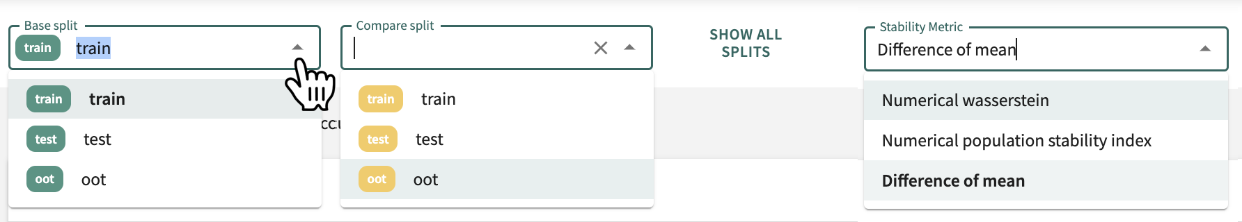
To deselect the Compare split, click SHOW ALL SPLITS.
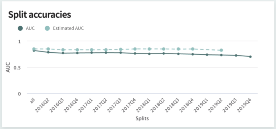
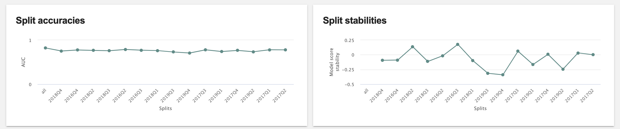
Split Accuracies and Drift (across splits)
When displayed at the top of the Drift page, these plots reflect model accuracy and stability (MSD), respectively, across splits relative to the baseline split. If the number of splits is limited, both graphs are hidden. If no ground truth data is available, the Split accuracies panel is hidden.
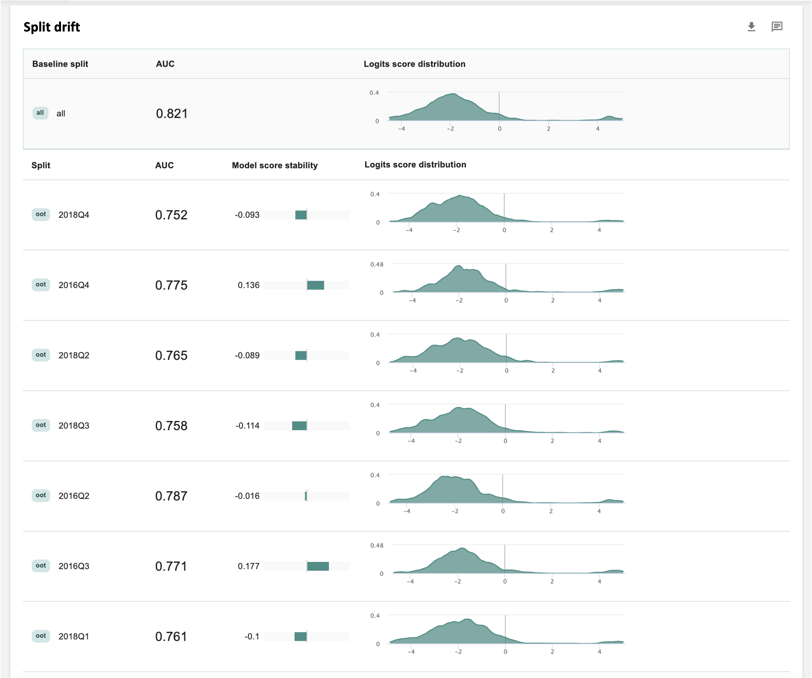
Split Drift (by split)
The Split drift panel displays the model's accuracy metric, MSD, and score distribution for all splits associated with the model. Baseline split scoring remains positioned at the top for comparison with the drift scores for all the splits below. Look for the highest and lowest MSD scores to identify splits that are behaving differently than your baseline split.
Base Split vs. Compare Split (split comparison)
For a one-to-one comparison of train/test splits with an OOT distribution, you'll need to select an OOT distribution as the Compare split. When you do, the drift scoring comparison in the top panel is organized into three comparison tabs — MODEL SCORE INSTABILITY, PERFORMANCE COMPARISON, and DATA COMPARISON.
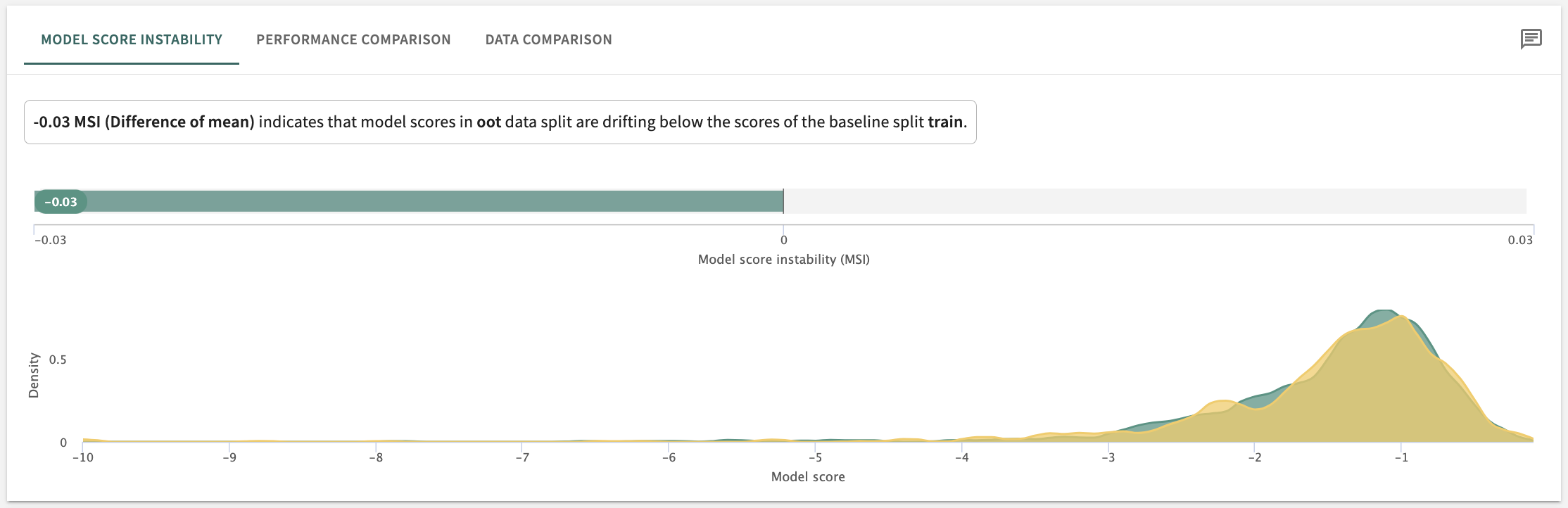
The score and what it indicates vis-à-vis model drift is summarized near the top of the panel. In the example captured above, the comparison of an oot split to the base split train measured in Difference of mean produced the drift indication shown, i.e., that model scores in the Compare split are drifting below those in the Base split (training).
Additionally, each of these comparison tabs can be extended by selecting a different drift metric.
Assessing Feature Drift
As with base vs. compare, a deep dive into feature drift requires you to focus on the MSD differential of just two splits at a time. Here, the comparison is organized into three tabs called CONTRIBUTION TO SCORE DRIFT, CONTRIBUTION TO ERROR REPORT, and FEATURE VALUE DRIFT. Each tab's analysis can also be extended by changing the drift metric.
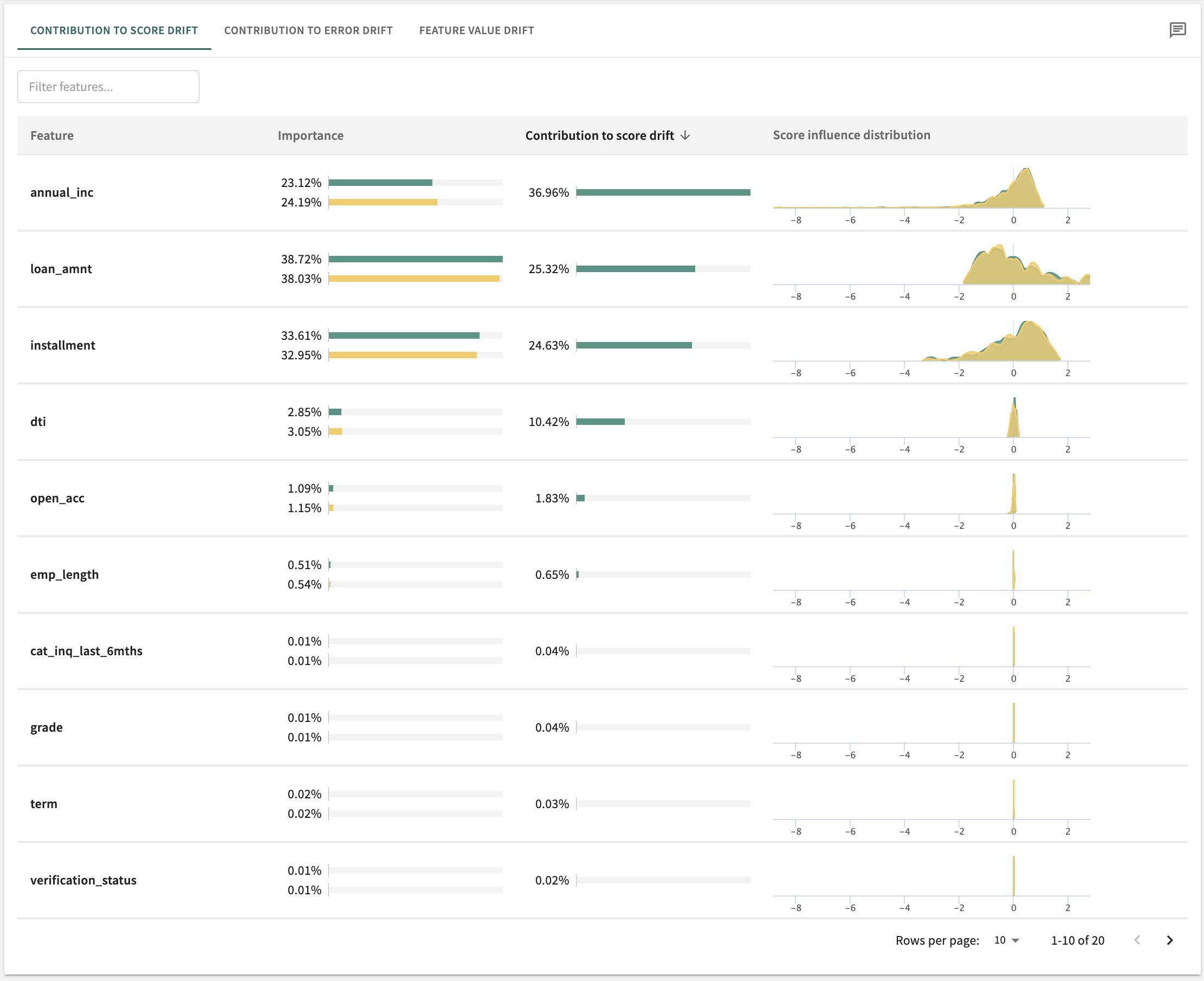
You can toggle the sort order of the list by column heading according to:
- Feature – alphabetically
- Importance – Difference, Base split: high to low and low to high, Compare split**: high to low and low to high
- Contribution to score drift – Absolute value, logistic contribution to score drift: high to low and low to high
To take a deep dive into specific feature, click on anywhere on its row.
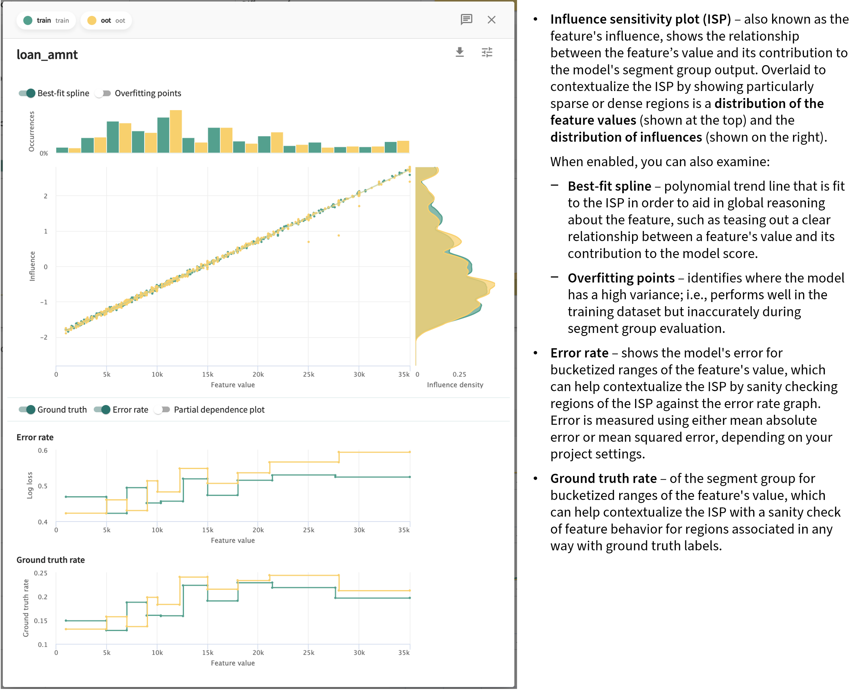
These plots show the change feature behavior across the two splits with respect to:
- Data distribution shift over the two time periods
- Change in the dependence of the model's output on the feature's value over time
- Change in feature contribution of the model's output.
Creating Drift Reports
Once you've generated an online drift analysis based on a desired model, splits, and drift metric, you can capture the results in a formal report that's download-ready in an editable .docx format for offline review and publication.
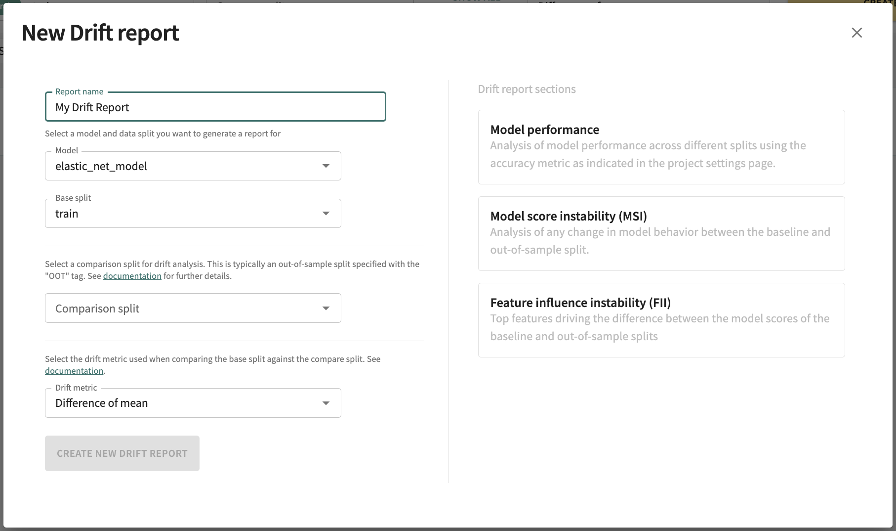
 To generate the report, click CREATE DRIFT REPORT near the top of the Drift page. This opens a New Drift Report form you can complete by adding a Report Name and confirming/changing the drift analysis parameters.
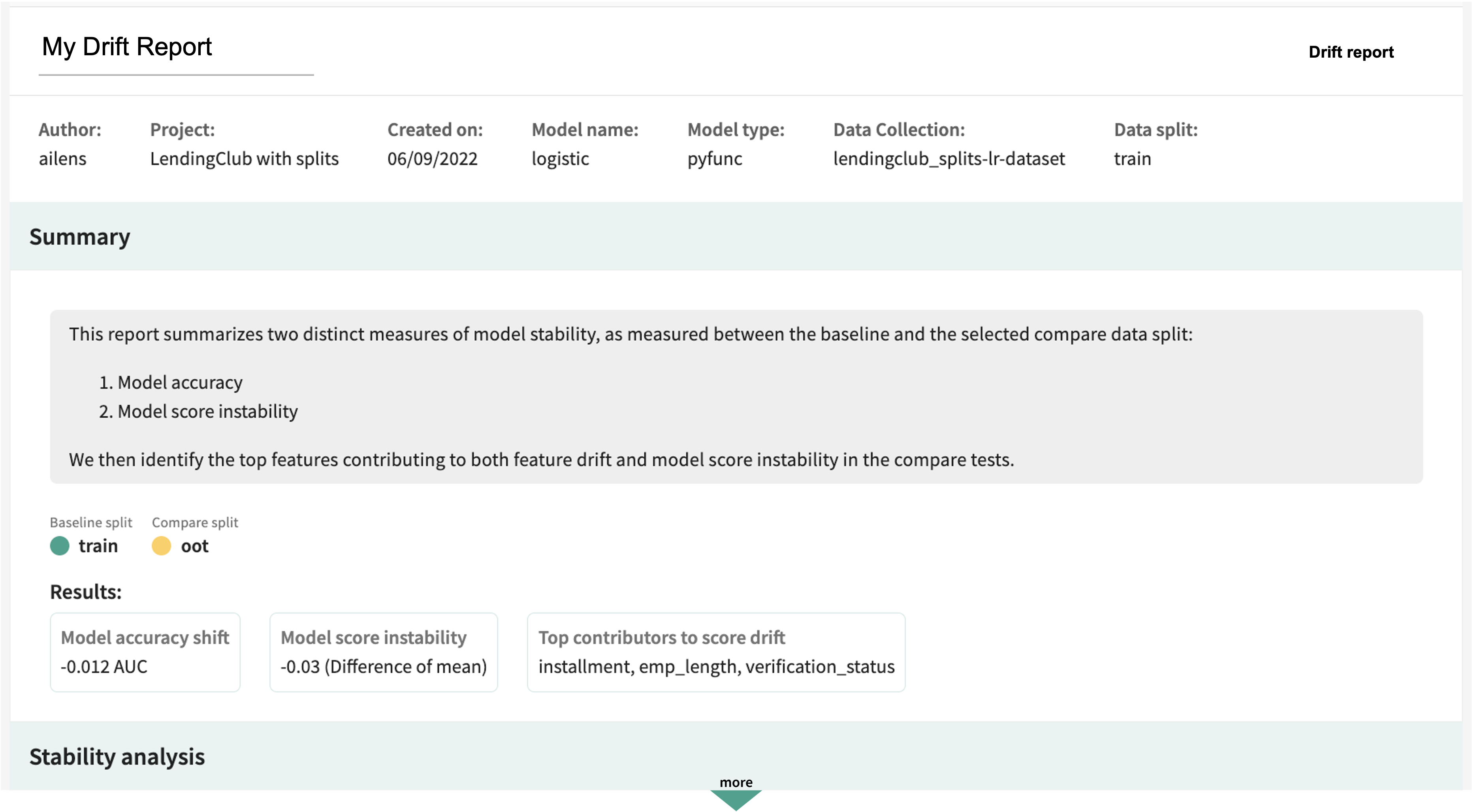
Click CREATE NEW DRIFT REPORT at the bottom-left of the form to generate the report, which will be formatted similarly to the following, with a header specifying the title, creation date, project, model, model type, data collection, and split. This is followed by a summary of the results.
Consistent with the assessments described in the guidance above, the analysis itself is organized into the following general sections:
- Model performance
- Model Score Instability (MSD)
- Feature Influence Instability (FID)
- Drift details for each feature
Each section and feature detail can be included/excluded using the on/off toggle at the top of the respective section/feature. A Notes field is also provided in each section to enter your comments, insights, questions, and feedback. Again, after download to a .docx file, you can edit all areas of the report as desired.
To export/download the report, click Export in the top right of the on-screen report.

Click Next below to continue.
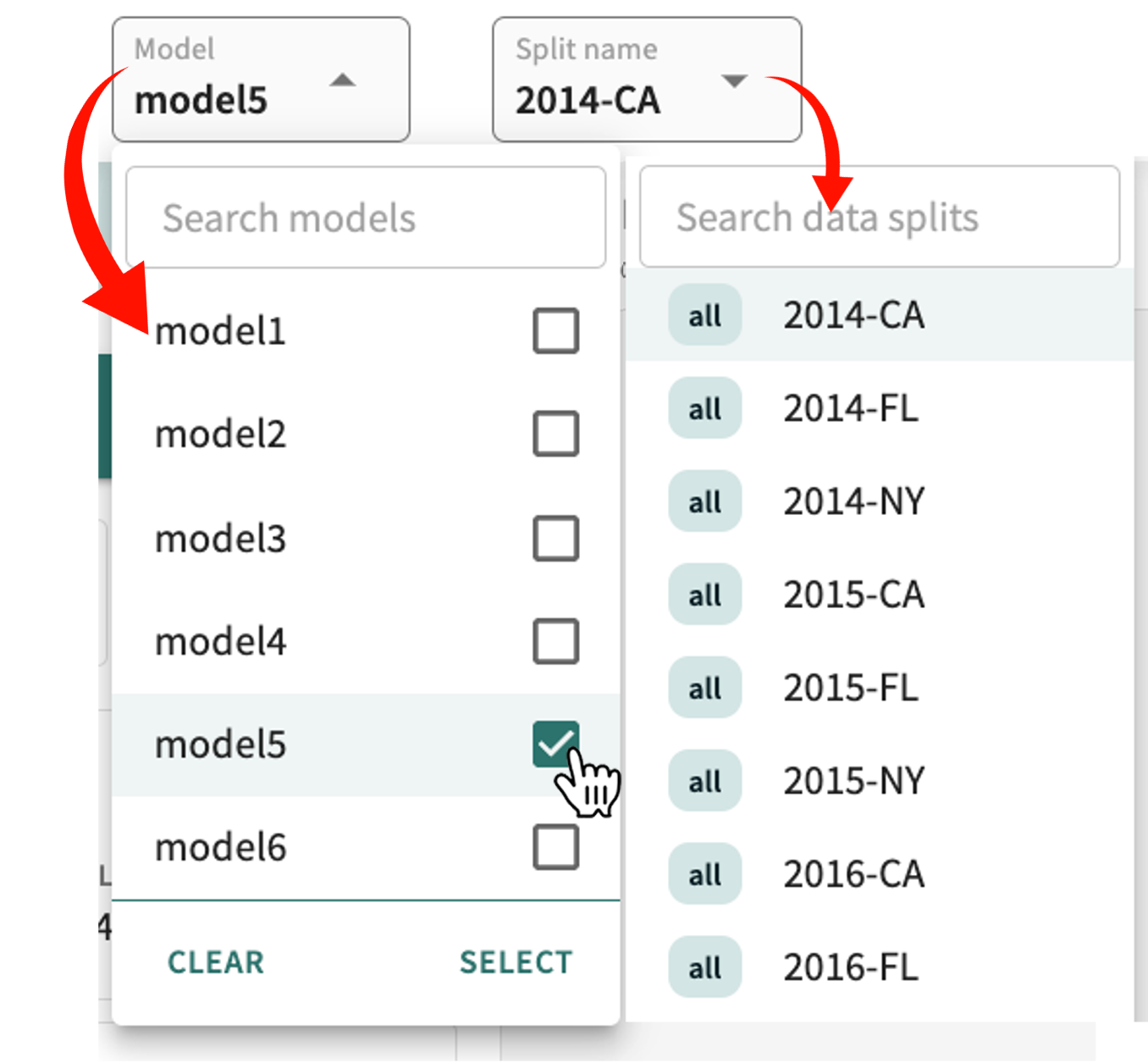
- Click the Model selector.
- Deselect the currently selected model(s), then select the desired model(s).
- Click SELECT.
- Click the Split name selector.
- Select the desired split.
Search for a model or split by entering a parial or full string in the respective search box.
- Click the Drift metric selector.
- Select the desired metric.